Designing Synthesizable Ionizable Lipids with Generative Models
A deep dive on synthesis-constrained discrete diffusion — the math of diffusing over molecular graphs, why we freeze the reaction scaffold, how region-aware noise fixes the chemistry, and what came out the other side.
The ionizable lipid is the molecule at the heart of a lipid nanoparticle — the part that grabs an mRNA or gene-editing payload and carries it into the cell — and it's still discovered largely by trial and error over human-designed libraries. This is a walkthrough of what it takes to generate them instead, with the equations and the failure modes shown rather than skipped. It covers our work, Synthesis-Constrained Discrete Diffusion for Ionizable Lipid Generation (with Rohin Maganti and Mohamad-Gabriel Alameh).
The one-paragraph version. Ionizable lipids are discovered by enumerating combinatorial libraries; existing machine learning only ranks those libraries. We build the first generative model for ionizable lipids, using discrete diffusion over molecular graphs. The trick is that the combinatorial reaction that makes these lipids fixes part of the molecule deterministically, so we hold that part constant during diffusion and generate only what the chemistry leaves free. Every sample is synthesizable by construction. In our experiments, 99% of generated lipids are chemically valid with an intact scaffold, 62% are novel, and the best candidate has roughly  the predicted transfection potency of the training-set mean.
1 · What an ionizable lipid is, and why generation is hard
A lipid nanoparticle (LNP) is the delivery vehicle behind the mRNA COVID vaccines and a growing list of genetic medicines. Its functionally decisive component is the ionizable lipid: it complexes the negatively charged mRNA, and it's the reason the payload escapes the endosome. The chemistry that makes this work is a pKa trick — the lipid is close to neutral at physiological pH ( ), so it doesn't wreck membranes in circulation, but it protonates in the acidifying endosome, becomes cationic, and drives escape into the cytosol.
The ionizable lipid never works alone. A finished LNP is a four-component formulation — the ionizable lipid, a helper phospholipid, cholesterol, and a PEG-lipid — self-assembled with the RNA at fixed molar ratios, and the particle's behavior depends on that whole recipe and the mixing process, not on the lipid in isolation. But among the four, the ionizable lipid is the one that carries the charge and does the escaping, and small changes to it move potency and tolerability the most. The single number that matters most is its apparent  : too basic and the particle stays cationic in circulation, where it is cleared quickly and is toxic; too acidic and it never protonates in the endosome to trigger escape. The empirical sweet spot for delivery to the liver sits near 6.5, and where a lipid lands is a matter of head-group and linker chemistry — exactly the part a generator gets to choose.
Structurally, an ionizable lipid has three kinds of region: a nitrogen-containing head, two lipophilic tails, and the core (linker) that joins them. Those regions have very different chemistry, and that difference turns out to be the whole game.
Today these lipids are found by combinatorial chemistry — pick building blocks, react them, screen the products — and the machine learning layered on top is discriminative: featurize the enumerated library, train a predictor of transfection potency, rank. That's useful but bounded: you can only rank molecules someone already drew, and the space of synthesizable lipids dwarfs any library. We wanted the model to propose lipids nobody enumerated.
How bounded is "rank the library"? The published discriminative models — AGILE and LiON among them — are trained on libraries ranging from a few thousand to about twelve thousand lipids, while the space of ionizable lipids reachable from commercial building blocks runs into the billions. A ranker can only return the best of what it was shown; it cannot point outside the enumeration. If the best possible lipid isn't in your library, no amount of ranking will find it. Generation is the attempt to leave the library behind and sample from the far larger space of things that could be made but never were.
The obvious move — take a generic molecular generator and point it at lipids — fails in two ways. It emits chemically invalid graphs (bad valences, unparseable structures), and it emits valid-but-unmakeable ones. Lipid chemistry has its own grammar (tertiary-amine heads, long branched alkyl tails, ester/amide linkers) that looks nothing like the drug-like molecules these models train on. The problem is not the architecture. It's that the constraints of real lipid chemistry have to live inside the generator.
The mismatch is concrete. Drug-like training sets like ZINC center on molecules of roughly 300–500 daltons, with short and often aromatic scaffolds and single-digit logP; an ionizable lipid is 700–800 daltons, carries two saturated tails a dozen or more carbons long, and has a logP up in the teens. A model that has only ever seen the former treats the latter as wildly out-of-distribution, and it fails in the two ways above — invalid graphs and unsynthesizable ones — because nothing in its training taught it that a lipid is a specific, makeable kind of object. Everything that follows is about putting that knowledge into the model instead of hoping it emerges.
2 · Background: discrete diffusion on molecular graphs
A molecule is a graph  :
:  atoms with categorical types
  (C, N, O, S, …) and bonds with categorical types
  (none, single, double, triple, aromatic). Because everything is categorical rather than continuous, we can't add Gaussian noise the way image diffusion does. We use discrete diffusion (Austin et al., 2021; Vignac et al., 2023).
| Symbol | Meaning |
|---|---|
| molecular graph: atom types  , bond types , bond types |
 | number of atoms; number of categories (atom/bond types) |
 | single-step forward transition matrix |
 | prior (limiting) distribution; region-specific prior for region  |
 | per-step noise rate; cumulative signal retained to step  |
 | graph-neural-network denoiser |
 | indices of the fixed core (scaffold) atoms and bonds |
 | target property (transfection potency); guidance scale |
Why diffusion, and why discrete
Molecular generation has been tried with most of the generative toolkit: variational autoencoders over SMILES or junction trees (Gómez-Bombarelli et al., 2018; Jin et al., 2018), autoregressive graph models, normalizing flows, and GANs. Diffusion has become the default for graphs because it sidesteps the others' failure modes at once — it needs no fixed generation order (autoregressive models impose an arbitrary atom ordering), no invertibility constraint (flows do), and it trains by denoising rather than by adversarial min-max (GANs are unstable). For a problem where chemical validity and diversity both matter, that combination is hard to beat.
The wrinkle is that a molecular graph is categorical — atom types and bond orders are discrete labels, not points in a continuous space — so the Gaussian noise that drives image diffusion has no natural meaning here, and rounding a continuous relaxation back to discrete atoms introduces its own artifacts. Discrete diffusion (Austin et al., 2021) defines the corruption directly on the categorical variables, which is what makes it the right tool.
Take a single categorical variable  as a one-hot row vector. The forward process corrupts it one step at a time by mixing in a prior
  (a distribution over the
  categories):

Here ![\beta_t \in [0,1]](../assets/math/synthesis-constrained-diffusion-m20.svg) is the noise rate at step . Reading the transition matrix: with probability
is the noise rate at step . Reading the transition matrix: with probability  the category is left alone, and with probability
  it is resampled from the prior
  . Because the single-step matrices share this structure, the -step cumulative transition has a closed form,

which gives a direct sampling formula — jump straight from the clean value to any timestep without simulating the chain:

As  ,
,  and the variable forgets its origin:
  . For a whole graph, atoms and bonds are corrupted independently, so the forward distribution factorizes:

Training a generator means learning the reverse process. A neural denoiser  — a graph neural network — looks at the corrupted graph and predicts the clean categorical types of every atom and bond. At sampling time you start from pure noise
  and walk backward to
  .
.
Two design choices in that sketch are worth naming. First, the prior : discrete diffusion can corrupt toward a uniform distribution, toward a special absorbing "mask" state, or toward the data's own marginal type distribution. We use the marginal — the empirical frequency of each atom and bond type in the data — so that the fully-noised graph already has roughly the right composition (mostly carbon, a little nitrogen and oxygen) rather than an unnatural uniform soup. The denoiser then has less distance to travel back to the data manifold. It is also the choice the region-aware noise in §4.2 refines.
Second, what the denoiser predicts. Rather than predict the small per-step change, predicts the clean graph directly — the " -parameterization" — and the reverse step is obtained by plugging that prediction into the posterior
  , which is available in closed form because the forward chain is a known Markov process. Predicting keeps the training target stationary across timesteps and lets the model reason about the whole molecule at once instead of a local nudge. The network is a graph neural network that is permutation-equivariant — relabel the atoms and its predictions relabel with them — which is exactly the symmetry a molecule needs, since a graph carries no canonical atom order.
until the graph is pure noise; the learned denoiser runs the chain backward. Grey marks corrupted variables.The training objective
Like other diffusion models, discrete diffusion is trained to maximize a variational lower bound on the data log-likelihood. Written over timesteps, the bound splits into a reconstruction term, a sum of per-step KL divergences between the true posterior and the model's, and a prior term that is constant in  :
:
![\mathcal{L}_{\mathrm{vb}} = \mathbb{E}_q\!\left[\, -\log p_\theta(G_0 \mid G_1) \;+\; \sum_{t=2}^{T} \mathrm{KL}\!\big(q(G_{t-1}\mid G_t, G_0)\,\big\|\,p_\theta(G_{t-1}\mid G_t)\big) \;+\; \mathrm{KL}\!\big(q(G_T\mid G_0)\,\big\|\,p(G_T)\big) \,\right].](../assets/math/synthesis-constrained-diffusion-d4.svg)
Because the denoiser predicts directly and the posterior  is known in closed form, each KL term reduces to a comparison between two categorical distributions, and in practice the whole objective is optimized as a plain cross-entropy between the predicted clean types and the true ones — the scaffold-masked form of which appears in §4.1. Noise is added on a standard monotone schedule for that spends more steps in the low-noise regime, where reconstruction is hardest and most of the model's accuracy is won or lost.
3 · The observation: the reaction fixes part of the molecule
Combinatorial lipid libraries are built from multicomponent reactions. We build ours around the Ugi three-component reaction, which combines an amine, an aldehyde, and an isocyanide in one pot to form a bis-amide product (Ugi et al., 2000). The mechanism is deterministic where it counts: the same three reactant classes always produce the same scaffold topology. Varying the amine tunes the head; varying the aldehyde and isocyanide tunes the tails; the core bonds are formed by the reaction itself and never move.
Most generative approaches treat that determinism as something to rediscover from data. We treat it as free information. The Ugi core bonds are not statistical regularities to be learned — they're mechanistic invariants. So we take them out of the generative problem entirely. Formally, we define a scaffold as four things: the number of atoms (typically 40–49 for these lipids), the bond topology, a region assignment  , and the core bond types. Diffusion then only has to fill in atom types and the non-core bonds.
It's worth seeing why the core is genuinely invariant. In the Ugi reaction the amine and aldehyde first condense into an imine; the isocyanide adds to it, and a rearrangement stitches the fragments together through two amide bonds. Those bonds — the bis-amide core — are a consequence of the mechanism, not of which reactants you picked, so every product built this way shares the same central connectivity and differs only in the substituents hanging off it. Across the 1,100-lipid experimental set this produces 527 distinct scaffold topologies (and 7,620 across the 12,000-molecule virtual library): hundreds of fixed skeletons, each decoratable in many ways.
Contrast this with how synthesizability is usually enforced: generate freely, then score each molecule with a synthetic-accessibility heuristic or run a retrosynthesis engine to look for a route, and discard whatever fails. Both are post-hoc, both are approximate, and both waste the model's output — it spends capacity proposing molecules that get thrown away. Fixing the reaction scaffold inverts that. Every sample is, by construction, the product of a known one-pot reaction from commercial building blocks, so synthesizability is a guarantee rather than a filter. The cost is committing to one reaction's chemistry; the benefit is that nothing generated is wasted.
4 · Method
Three modifications turn a generic graph-diffusion model into a lipid-aware one: fixing the core, region-aware noise, and property conditioning.
4.1 · Fixing the core (scaffold conditioning)
Let  be the set of core atom (and bond) indices. We remove them from diffusion in two matching ways. During training, core positions are masked out of the loss — the denoiser is never asked to predict them, so it spends none of its capacity relearning the reaction mechanism. The objective becomes a cross-entropy over the free positions only:
![\mathcal{L} = \mathbb{E}_{t,\,G_0,\,G_t}\!\left[\ \sum_{i \notin \mathcal{C}} \ell\!\left(f_\theta(G_t, t)_i,\ G_0^{(i)}\right)\right].](../assets/math/synthesis-constrained-diffusion-d5.svg)
During generation, core bond entries are overwritten with the ground-truth scaffold after every denoising step, not just the last one, so scaffold corruption can't accumulate through the reverse chain. In the paper we show this restoration is exact under the factorized forward process — because atoms and bonds diffuse independently, clamping the core introduces no approximation into the posterior over the rest of the graph.
Mechanically, "the core" is found by matching the Ugi substructure pattern against each training graph, which labels the invariant atoms and bonds; those indices are . Holding them fixed while denoising the rest is a form of inpainting — the same move image diffusion uses to fill a masked region while keeping the known pixels. But image inpainting (as in RePaint) is only approximate: because pixels are coupled through convolutions, the known and unknown regions have to be repeatedly re-harmonized or the seam shows. Here the forward process factorizes over atoms and bonds — each is corrupted on its own — so conditioning on the core variables changes nothing about the posterior over the free ones. Clamping the scaffold at every step is therefore exact rather than approximate, which is what lets us apply it throughout the reverse chain without drift.
4.2 · Region-aware noise
This is the piece that matters more than it looks. Standard diffusion corrupts every atom toward one global prior . But an ionizable lipid is chemically lopsided — heads are nitrogen-rich, tails are almost pure carbon — so a single global prior forces the denoiser to fight a mismatch between the noise it sees and the data it must reconstruct. Instead we give each region its own transition matrix with its own stationary distribution  :
:

Head atoms diffuse toward a nitrogen-enriched prior (28% N versus 8% globally); tail atoms toward a carbon-dominated one (94% C). Each edge inherits the region of its source atom. The reverse posterior stays tractable: for an atom in region ,
![q\!\left(x_{t-1}=k \mid x_t=j,\, x_0=\ell;\, r\right) \ \propto\ Q_t^{(r)}[k, j]\ \cdot\ \bar Q_{t-1}^{(r)}[\ell, k].](../assets/math/synthesis-constrained-diffusion-d7.svg)
This has exactly the same algebraic form as the standard posterior with replaced by — same  cost per atom, no new approximation, just a different limiting distribution per region. All regions share one noise schedule
  ; only where they converge differs.
Why does the limiting distribution matter so much when it is just "where the noise ends up"? Because the denoiser's entire job is to invert the forward process, and the difficulty of that inversion depends on how far the noise drags the data off its own manifold. Corrupt a carbon-dominated tail toward a global prior that carries the head's nitrogen, and the reverse network has to spend capacity undoing nitrogen that never belonged there. Match the noise to each region's real composition and the forward process stays close to the data everywhere along the chain, so the reverse process faces an easier, better-specified problem. The region priors are, in effect, an inductive bias about local chemistry injected through the noise itself — the cheapest place to put prior knowledge, because it costs nothing at inference.
Why this earns its place. Ablate region-aware noise — use a single uniform prior — and the model produces 8% invalid molecules (versus 0% for the full model) and starts generating allenes and cumulenes: strings of cumulated double bonds like C=C=C=C=C that are chemically unstable and appear nowhere in the training data. Scaffold conditioning alone doesn't stop this. Without a prior that says "tails are lipophilic alkyl chains," the model wanders into implausible chemistry, because the global marginal can't tell a nitrogen-rich head from a carbon tail.
4.3 · Property conditioning
To steer toward activity, we inject a target transfection potency  into the denoiser through FiLM layers (Perez et al., 2018), which feature-wise scale and shift the intermediate representations, and we train with classifier-free guidance (Ho & Salimans, 2021) by dropping the conditioning signal 15% of the time. At sampling, we mix the conditional and unconditional predictions in logit space (empirically more stable than in probability space):

The guidance scale  interpolates between unconditional sampling (
 ) and aggressive steering toward the target (
 ), trading diversity for on-target potency.
A little more on each piece. A FiLM layer runs the conditioning value — here a single scalar, the target potency — through a small network into a per-channel scale  and shift
  , and applies
  to the denoiser's hidden features
  at each message-passing layer. It is a cheap, expressive way to let the target modulate every part of the network without touching its architecture. Classifier-free guidance then trains one model to do double duty: 15% of the time the conditioning is dropped, so the same weights learn both the conditional
  and the unconditional
  . At sampling, the guided prediction extrapolates along the direction from unconditional to conditional — geometrically, it reads off "which way makes this more like a high-potency lipid" and takes a larger step in that direction. Larger presses harder toward the target and narrows the output distribution; that is the diversity-for-fidelity trade, and it's why we report metrics across a sweep of rather than at one setting.
4.4 · The full sampling loop
Putting it together, generation proceeds in two stages. First, scaffold selection: because these lipids span hundreds of distinct scaffold topologies, we pick one by property-weighted sampling from a library extracted from the training data — scaffolds associated with high-potency molecules are more likely to be drawn. Second, diffusion: run the reverse chain to fill in the free atoms and bonds, applying guidance and restoring the scaffold at each step.
Algorithm 1 — Reaction-constrained diffusion sampling
input target property , guidance scale , diffusion steps 
- Initialize
 from the region-aware priors , and fix the core bonds
 ![E_T[\mathcal{C}] \leftarrow E_\mathcal{C}](../assets/math/synthesis-constrained-diffusion-m51.svg) .
. - For
 :
:
- Form the guided prediction

- For each region , sample from the region-specific posterior

- Restore the scaffold,
![E_{t-1}[\mathcal{C}] \leftarrow E_\mathcal{C}](../assets/math/synthesis-constrained-diffusion-m53.svg) .
.
- Form the guided prediction
- Return . The final step samples
 multinomially (not argmax) to preserve diversity.
5 · Training on almost no data
The binding constraint is data: only about 1,100 Ugi-based lipids have measured transfection. You cannot train a graph-diffusion model from scratch on 1,100 graphs. So we use a three-stage curriculum that walks the model from generic chemistry down to lipid activity, unfreezing capabilities as the distribution narrows.
The logic is that the three datasets teach different things at different resolutions, and cheap-but-plentiful data should teach the general skills before scarce-but-precise data teaches the specific ones. Stage 1 (ZINC250k, 250,000 drug-like molecules, ~500 epochs) teaches the grammar of valid chemistry — valences, ring closures, what a parseable molecule even is — with no notion of lipids at all. Stage 2 (the 12,000-molecule AGILE virtual library, ~300 epochs) switches on region-aware noise and scaffold conditioning and shifts the distribution onto lipids, teaching the model what heads and tails look like. Only Stage 3 (the ~1,100 measured lipids, ~300 epochs) introduces potency labels and the FiLM/guidance machinery. Sequencing it this way is also a hedge against catastrophic forgetting: each stage adapts a model that already works rather than training from scratch on data too small to support it, so the general chemical competence learned early is refined instead of overwritten.
6 · The generator and the oracle are kept apart
This is the design choice I'd most want a skeptical reader to notice, because it guards against the most common failure mode in model-guided design: a generator that learns to exploit the blind spots of its own scoring function. We score candidates with LANTERN (Mehradfar et al., 2025), a graph neural network trained on experimental transfection data that predicts measured transfection potency (mTP) with an  on held-out lipids. But the diffusion model does not optimize against LANTERN. It learns the distribution of structures in stages 1–2 with no property labels at all; LANTERN-corrected potency enters only as a conditioning target in stage 3, and at generation time LANTERN is used purely to rank finished samples after the fact.
The consequence is that the generator can't exploit blind spots in the predictor. It samples from a learned chemical distribution and the predictor grades the output; it never gets to descend the predictor's loss surface and find its adversarial holes. It also makes the oracle swappable — a better predictor, or a batch of real wet-lab measurements, can replace LANTERN without retraining the generative model. Decoupling the two is what keeps the in-silico search honest.
It's worth being precise about the failure this avoids, because it is the default outcome of the more obvious design. If you instead optimize a generator directly against the predictor — reinforcement learning with the predictor as reward, or Bayesian optimization over its surface — the optimizer's incentive is to find wherever the predictor is wrong in an optimistic direction. A predictor trained on ~1,000 noisy measurements has plenty of such holes, and a determined search will land in them, producing molecules the model scores as brilliant and the world scores as ordinary. Keeping the training signal (the data distribution) separate from the evaluation signal (the predictor) removes that incentive by construction: the generator has no gradient into LANTERN's mistakes because it never sees LANTERN's loss surface. The practical dividend is modularity — when we swap LANTERN for wet-lab measurements on the lipids we're now synthesizing, the generator doesn't change at all; only the oracle does.
7 · Results
We generated 100 molecules targeting mTP  at guidance scale
  and evaluated them. "Valid" means chemically valid (correct valence, parseable) and containing an intact Ugi scaffold.
| Metric | Value |
|---|---|
| Chemically valid | 99% |
| Ugi scaffold intact | 100% |
| Unique structures | 91% |
| Novel (not in training) | 62% |
| Mean predicted mTP | 5.37 |
| Best predicted mTP | 10.55 |
| Training mean mTP | 4.85 |
.Across a sweep of seeds and guidance scales the picture holds: above 90% validity, 100% scaffold integrity, and novelty between 60% and 73%. Novelty means absent from both the 12,000-molecule virtual library and the 1,100-molecule experimental set. Because standard Morgan fingerprints understate how different two lipids are, we re-checked with Atom-Pair fingerprints, which capture lipid topology better: 43% of the novel molecules have nearest-neighbor similarity below 0.95 — structurally distinct, not cosmetic edits.
| Seed | CFG | Validity | Novelty | Mean mTP |
|---|---|---|---|---|
| 0 | 1.0 | 96.7% | 60.4% | 5.54 |
| 0 | 2.0 | 93.3% | 60.2% | 5.58 |
| 0 | 3.0 | 96.7% | 65.4% | 5.61 |
| 1 | 1.0 | 96.7% | 70.2% | 5.04 |
| 1 | 2.0 | 93.3% | 63.4% | 5.69 |
| 1 | 3.0 | 76.7% | 74.2% | 4.77 |
| 2 | 1.0 | 98.3% | 70.6% | 4.62 |
| 2 | 2.0 | 98.3% | 60.9% | 5.41 |
| 2 | 3.0 | 96.7% | 72.6% | 5.33 |
The sweep also shows the guidance trade-off from §4.3 in the data: pushing up tends to raise novelty (the model wanders further from the training set) at some cost to validity — most visibly at seed 1,  , where validity drops to 77% while novelty climbs to 74%. We report at
  as a balance, but nothing here is knife-edge: every setting clears 90% validity except that one, and all keep the scaffold intact.
That fingerprint choice is doing real work, so it's worth unpacking. Exact-match novelty is weak — a one-atom change already counts as new — so what matters is how far each novel molecule sits from its nearest training neighbor. Morgan (circular) fingerprints emphasize local atom environments, which makes any two long-tailed lipids look similar because they share the same repeating methylene groups; by that measure almost nothing looks novel. Atom-Pair fingerprints instead encode the topological distance between pairs of atoms, so they separate lipids by overall architecture rather than by their shared greasy tails. Reading novelty through the stricter, more appropriate lens is what turns "62% not seen before" into the stronger claim that nearly half of those are genuinely different skeletons.
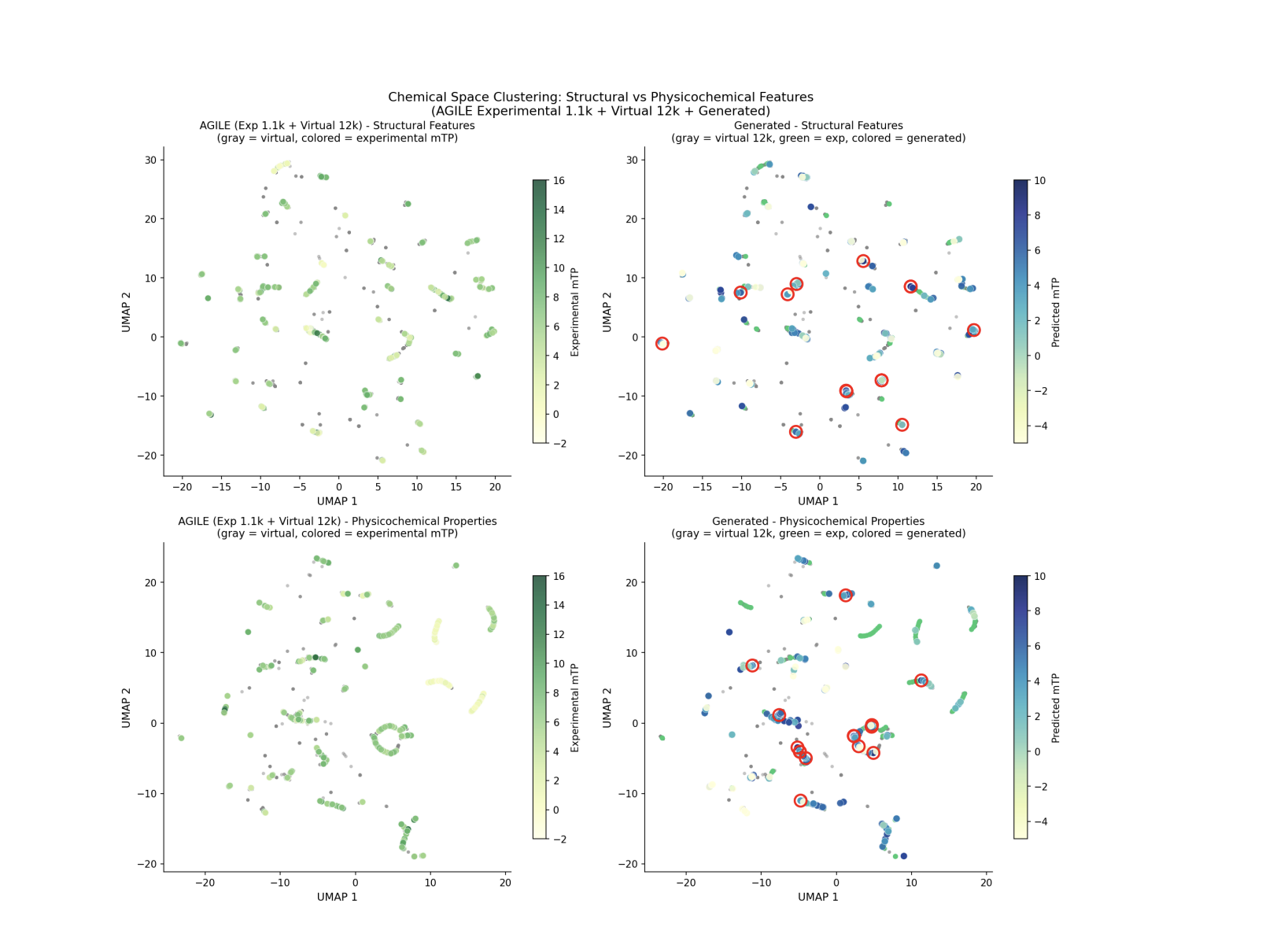
Two analyses I trust more than the headline numbers:
Where the potency variance lives. An ANOVA-style decomposition on the training data shows scaffold identity explains about 65% of the variance in transfection potency, and within-scaffold chemical variation explains the other 35% — a large space that library enumeration samples only sparsely (median within-scaffold potency range of 6.2 points). Our two-stage design maps onto this directly: property-weighted scaffold selection captures the 65%, and diffusion optimizes within the selected scaffold to capture the 35%.
Convergent design. Despite being novel, the top candidates agree with each other. The top three all carry dibutylamine heads — a minority motif in the training data — and the top seven share a topological polar surface area of 71 Ų and two hydrogen-bond donors, with tails in the C12–C16 range. A model that had merely memorized would not rediscover a rare-but-good head group and concentrate on it; converging on shared motifs it wasn't handed is evidence it learned something about structure and activity.
And the motifs are chemically legible, which is part of why they reassure rather than alarm. A dibutylamine head is a compact, moderately basic tertiary amine — the kind of group that lands the apparent near the escape-competent window; a topological polar surface area around 71 Ų with two hydrogen-bond donors matches the hydrogen-bonding pattern seen in effective ionizable lipids; and C12–C16 tails (the best candidate carries an unsaturated C18) sit squarely in the range that packs into stable particles without being too rigid. None of this was handed to the model as a constraint. Measured against the discriminative baselines on capability rather than on a single number, the gap is categorical: AGILE and LiON predict activity and are synthesizable only by staying inside their libraries, whereas this model generates novel structures, is property-conditioned, and stays synthesizable by construction — it explores beyond the enumeration instead of ranking within it.
| Rank | mTP | MW | LogP | TPSA | HBD | Novel |
|---|---|---|---|---|---|---|
| 1 | 10.55 | 790 | 14.2 | 71 | 2 | yes |
| 2 | 9.56 | 694 | 11.7 | 71 | 2 | yes |
| 3 | 9.01 | 788 | 13.6 | 71 | 2 | yes |
| 4 | 8.58 | 622 | 9.5 | 71 | 2 | yes |
| 5 | 8.18 | 638 | 10.0 | 71 | 2 | yes |
| 6 | 8.00 | 708 | 11.9 | 71 | 2 | yes |
| 7 | 7.89 | 706 | 11.9 | 71 | 2 | yes |
| 8 | 7.87 | 547 | 8.2 | 96 | 3 | yes |
| 9 | 7.83 | 743 | 13.7 | 96 | 3 | yes |
| 10 | 7.81 | 662 | 11.1 | 71 | 2 | yes |
| 11 | 7.70 | 706 | 11.8 | 71 | 2 | no |
| 12 | 7.64 | 741 | 13.5 | 96 | 3 | yes |
| Capability | AGILE | LiON | This work |
|---|---|---|---|
| Predict activity | yes | yes | yes |
| Generate novel structures | no | no | yes |
| Guaranteed synthesizability | library | library | by construction |
| Property-conditioned | no | no | yes |
| Explore beyond enumeration | no | no | yes |
8 · What this doesn't do
It's in silico. Everything above is scored by LANTERN at . Until these lipids are synthesized and measured, the gains are predictions, not results. We're currently making lead candidates for validation in hepatocyte transfection and mouse biodistribution.
Fixing the scaffold caps diversity. Guaranteeing synthesizability by freezing the Ugi core means the model explores within Ugi-accessible space and cannot invent a fundamentally new reaction scaffold. That's a deliberate trade. The principle extends to other multicomponent reactions (Passerini, Biginelli, Hantzsch), each opening its own region of makeable space — but it is a ceiling, not an escape from one.
In vitro ≠ in vivo. Transfection in a dish correlates imperfectly with delivery in an animal, which depends on formulation, biodistribution, and immunogenicity the model never sees. No in-silico oracle escapes that gap; it only narrows it.
The path forward is the loop that makes any of this real: generate, synthesize the top hits, measure them, and feed the measurements back as new conditioning data — active learning rather than one-shot generation — plus multiple scaffold types and multi-property conditioning on pKa, logP, and clearance so the objective is more than potency. But the core claim already stands: if you constrain a generative model to the chemistry a reaction actually permits, you get novelty and synthesizability at the same time, instead of trading one against the other.
9 · Related work
Discriminative models for LNPs. The closest prior work predicts activity for pre-enumerated lipids. AGILE (Xu et al., 2024) and LiON (Witten et al., 2025) train neural networks to rank library candidates by transfection efficiency, and LANTERN (Mehradfar et al., 2025) — the oracle we borrow for evaluation — predicts transfection potency from structure. All three are bounded by their libraries; none propose new molecules. Our contribution is orthogonal to theirs: a better predictor makes a better oracle, but only a generator can leave the library.
Generative models for molecules. On the modeling side we build on discrete graph diffusion — D3PM (Austin et al., 2021) and DiGress (Vignac et al., 2023) — with classifier-free guidance (Ho & Salimans, 2021) and FiLM conditioning (Perez et al., 2018). The VAE and junction-tree generators (Gómez-Bombarelli et al., 2018; Jin et al., 2018) established the lineage; the scaffold-fixing trick is closest in spirit to diffusion inpainting (Lugmayr et al., 2022), made exact here by the factorized forward process rather than approximated by resampling.
Generative models for lipids. Two recent efforts target ionizable lipids specifically, both by searching over building blocks: a Monte-Carlo tree search over fragment libraries (Zhao et al., 2024) and a building-block DAG generator (Ou et al., 2024). Because they compose known fragments, they inherit the enumeration bottleneck they set out to escape. Learning the distribution of structures directly — while constraining generation to a reaction's makeable space — is what separates the approach here, and it is why synthesizability can be a guarantee instead of a fragment vocabulary.
References
Austin, Johnson, Ho, Tarlow & van den Berg. Structured denoising diffusion models in discrete state-spaces. NeurIPS 2021.
Vignac et al. DiGress: discrete denoising diffusion for graph generation. ICLR 2023.
Ho & Salimans. Classifier-free diffusion guidance. NeurIPS Workshop 2021.
Lugmayr et al. RePaint: inpainting using denoising diffusion probabilistic models. CVPR 2022.
Perez, Strub, de Vries, Dumoulin & Courville. FiLM: visual reasoning with a general conditioning layer. AAAI 2018.
Gómez-Bombarelli et al. Automatic chemical design using a data-driven continuous representation of molecules. ACS Central Science, 2018.
Jin, Barzilay & Jaakkola. Junction tree variational autoencoder for molecular graph generation. ICML 2018.
Ugi et al. Multicomponent reactions in organic chemistry. Angew. Chem. Int. Ed., 2000.
Coley et al. A robotic platform for flow synthesis of organic compounds informed by AI planning. Science, 2019.
Sterling & Irwin. ZINC 15 — ligand discovery for everyone. J. Chem. Inf. Model., 2015.
Cullis & Hope. Lipid nanoparticle systems for enabling gene therapies. Molecular Therapy, 2017.
Xu et al. AGILE: a deep-learning approach to accelerate LNP development for mRNA delivery. Nature Communications, 2024.
Witten et al. Artificial intelligence-guided design of lipid nanoparticles for pulmonary gene therapy. Nature Biotechnology, 2025.
Mehradfar et al. LANTERN: a machine-learning framework for LNP transfection-efficiency prediction. arXiv:2507.03209, 2025.
Ou et al. A deep generative model for the design of synthesizable ionizable lipids. NeurIPS Workshop, 2024 (arXiv:2412.00928).
Zhao et al. Generative model for synthesizing ionizable lipids: a Monte Carlo tree search approach. NeurIPS Workshop, 2024 (arXiv:2412.00807).
Maganti, Maganti & Alameh. Synthesis-constrained discrete diffusion for ionizable lipid generation. 2026.
Cited as
Maganti, Rahul. "Designing Synthesizable Ionizable Lipids with Generative Models." rahulmaganti47.github.io, July 2026.
@misc{maganti2026constrain,
  title  = {Designing Synthesizable Ionizable Lipids with Generative Models},
  author = {Maganti, Rahul},
  year   = {2026},
  url    = {https://rahulmaganti47.github.io/writing/synthesis-constrained-diffusion.html}
}